Principal Component Analysis

Principal Component Analysis (PCA) is a powerful dimensionality reduction technique that reduces the number of features (dimensions) while retaining the maximum variance in the data. By capturing the most important patterns in fewer components, PCA enhances data visualization and simplifies analysis.

We will now apply PCA to our filtered dataset and plot the resulting components to explore potential associations with study conditions. We will apply this transformation on filtered species. The code below perform that step.

import pandas as pd
from sklearn.decomposition import PCA
from sklearn.preprocessing import StandardScaler
import matplotlib.pyplot as plt
import seaborn as sns

# log transformed data from the previous step
df = microbiome_log

# Step 1: Standardize the data
scaler = StandardScaler()
scaled_data = scaler.fit_transform(df)

# Step 2: Apply PCA (reduce to 10 components for visualization)
pca = PCA(n_components=10)
pca_result = pca.fit_transform(scaled_data)

# Step 3: Create a DataFrame for PCA results
pca_df = pd.DataFrame(pca_result, columns=['PCA1', 'PCA2','PCA3', 'PCA4','PCA5',
                                           'PCA6','PCA7', 'PCA8', 'PCA9', 'PCA10'])

pca_df['study_condition'] = zeller_db['study_condition'].values

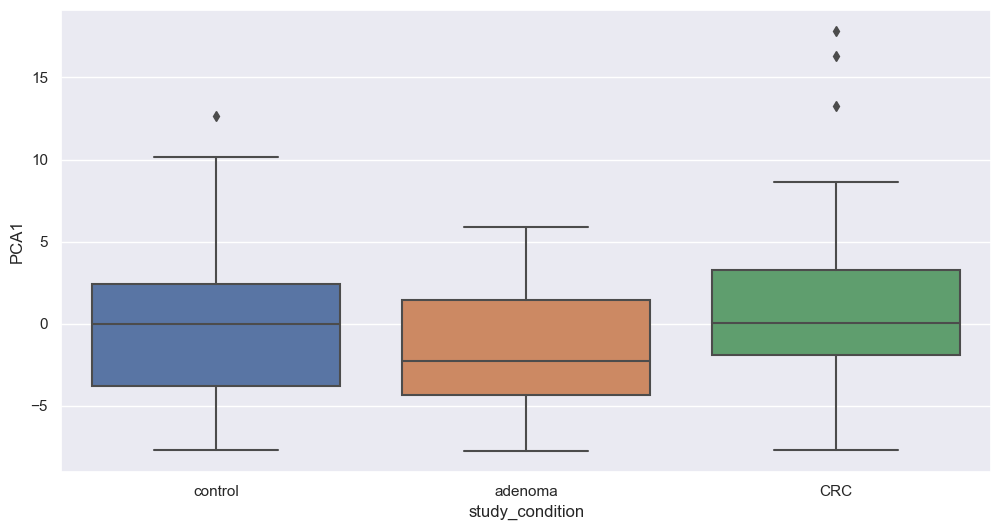
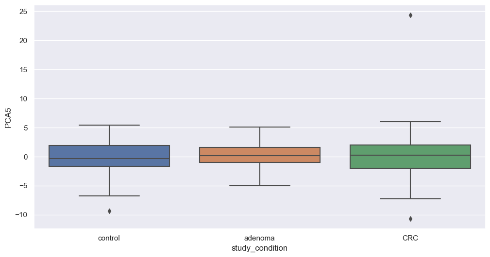
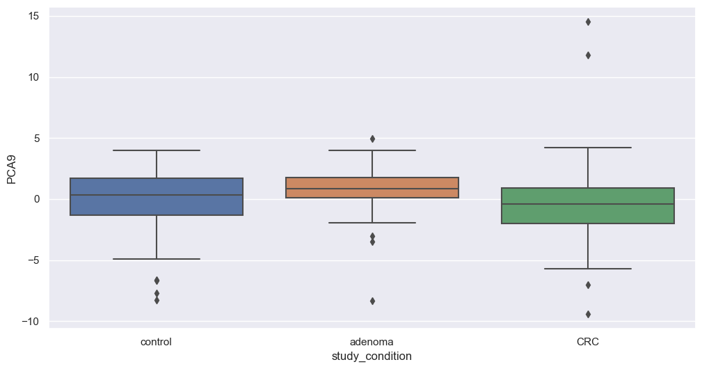
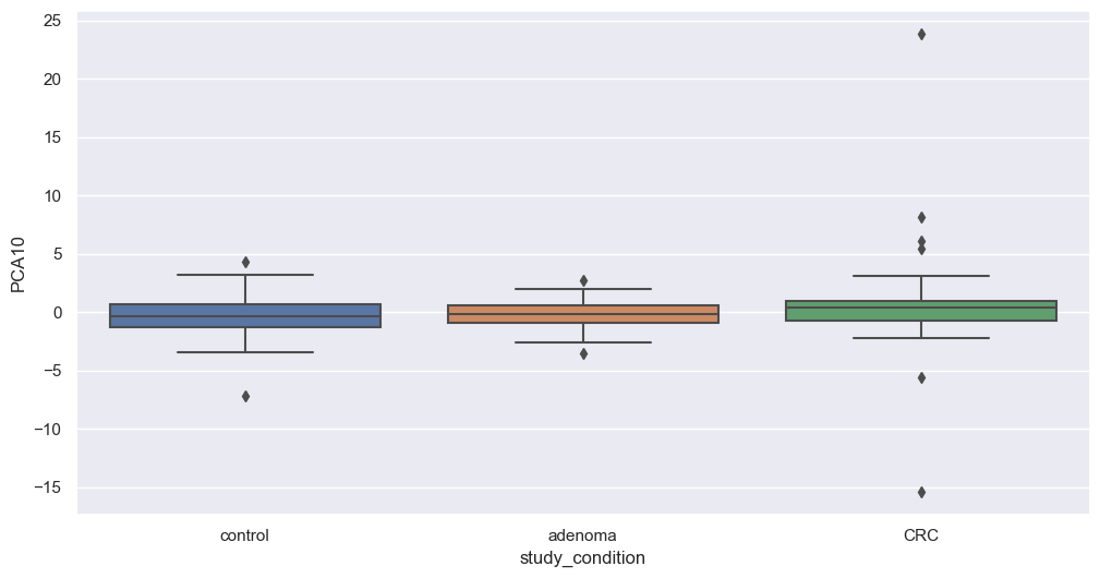
Figure fig-var below shows the cumulative variance captured by 10 principal components, i.e. 26%.

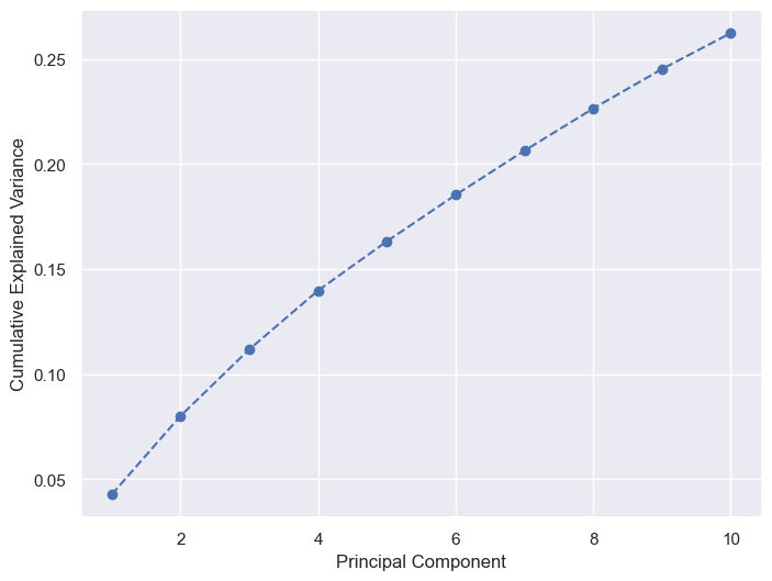
Figure 2: Cumulative Explained Variance by Principal Components

We will utilize PCA components in our modeling phase to build a CRC detection system.