In this post, I will give an introduction to Probabilistic Graphical Models in simple terms. By the end of this post, you will get an understanding of what PGM is, why probability is needed, and how graphical models help.
I have structured this post in three short subsections.
- Model
- Probabilistic Model
- Probabilistic Graphical Model
Model
Let’s begin with understanding the term “Model”. We can think about “Model” as a representation of our understanding of how things work in the world. For example, based on past experiences, a child might have a model like the one below for handling fire. The model below represents the child’s knowledge gained from our personal encounters with fire.
A model is a representation of our understanding of how things work; it encodes concepts and relationships but not the mechanism to reason about them.
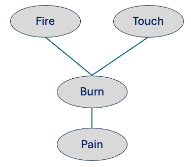
This is a declarative representation (Koller & Friedman, 2009) which describes What is, not how to compute. For example, the model above only captures key concepts (e.g., fire, touch, etc.) and relationships between them. To utilize this representation for reasoning a separate mechanism needs to be employed, and this is a key characteristic of this representation of the model (Koller & Friedman, 2009).
Probabilistic Model
Let’s consider an example to understand the role of probability here.
Imagine a team of doctors came up with an innovative surgery that can cure disease X. The team performed the surgery on 100 cases and was successful in 85 cases. The surgery was not 100% successful, which means its outcome can go either way. So there is some uncertainty over the result of the surgery, and the question is what is this some.
Formally, probability assigns numbers to events to quantify uncertainty and to support decisions.
A patient, who was recently diagnosed with disease X, learned about the surgery and contacted the team. The team will share this data that the surgery tends to have an 85% chance of being successful based on past experiences with similar cases (e.g., cases with a similar age group, lifestyle).
As you can see here, probability captures the uncertainty aspect and helps the patient to take into consideration available information for better decision-making.
We can write the notation in mathematical form using the given expression. Here, we are using three characteristics (i.e., whether the patient has a family history of the disease X, has an active lifestyle, and consumes the required nutrients) to compute the chances of successful surgery.
\[ P(S,F,E,N) \] (S = success, F = family history, E = Exercise, N = Nutrient)
For simplicity’s sake, I am considering variables as binary variables. For the computation of the above expression, we need a probability table consisting of probabilities for each choice of variables. In this case, we need probability values for 16 entries given in the table below.
| F | E | N | S |
|---|---|---|---|
| 0 | 0 | 0 | 0 |
| 0 | 0 | 0 | 1 |
| 0 | 0 | 1 | 0 |
| 0 | 0 | 1 | 1 |
| 0 | 1 | 0 | 0 |
| 0 | 1 | 0 | 1 |
| 0 | 1 | 1 | 0 |
| 0 | 1 | 1 | 1 |
| 1 | 0 | 0 | 0 |
| 1 | 0 | 0 | 1 |
| 1 | 0 | 1 | 0 |
| 1 | 0 | 1 | 1 |
| 1 | 1 | 0 | 0 |
| 1 | 1 | 0 | 1 |
| 1 | 1 | 1 | 0 |
| 1 | 1 | 1 | 1 |
For N variables of binary choices, the table grows exponentially to \(2^N\). In real-world problems, the choices can be more than 2, and that even further increases the table size. This poses challenges in managing & updating those tables.
Probabilistic Graphical Model
Graphical models solve the problem of huge probability tables by drawing the relationships between variables. Instead of one giant table with every possible combination, a PGM breaks the problem into small pieces and shows which variables directly affect which others. That makes the whole model much smaller and easier to work with.
Think of a PGM like a wiring diagram for uncertainty: each circle (node) is a variable (e.g., Success, Family history, Exercise, Nutrient) and each arrow or line shows a direct influence. Because the graph tells you who depends (or is influenced) on whom, you only need to store a small table for each node that says “given my parents, what are my chances?” — these are called conditional probability tables (CPTs) for directed graphs.
Two common kinds of PGMs:
- Bayesian networks (directed): arrows show direction of influence (good for cause→effect stories).
- Markov networks (undirected): lines show mutual relationships without direction.
Why does this help?:
- Much smaller tables: you store many small local tables instead of one enormous one.
- More intuitive: the picture shows the important relationships at a glance.
- Reusable and local: you can update or learn from one local table without rebuilding everything.
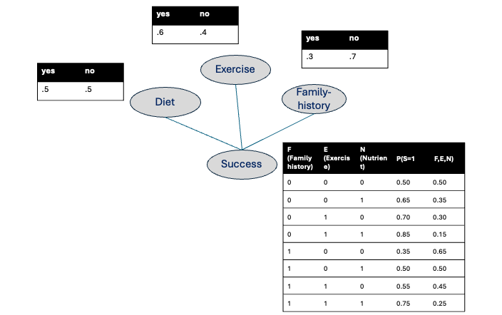
Surgery example: instead of listing probabilities for every possible combination of family history, exercise, nutrients, and success (2^4 = 16 entries), a graphical model stores a CPT for Success given its direct causes and separate simple tables for the other variables — often far fewer numbers overall. Algorithms (exact or approximate) then use these local tables plus the graph to compute the probabilities you care about.
I hope you find this post helpful in understanding PGM.
References
- Koller, D., & Friedman, N. (2009). Probabilistic graphical models: principles and techniques. MIT Press.