This post offers an introduction to discrete data distributions which are essential to know for every data scientist. The post starts by explaining what does it mean by data distribution and then dives deep into the following six data distributions with real world examples:

Bernoulli
Binomial
Geometric
Negative binomial
Hypergeometric
Poisson

What is data distribution?

Let’s now understand what is the meaning of data distribution. In data science projects, we work on different types of data and those data come from somewhere. For example, a dataset containing salary information of employees comes from a population of employees working at a particular company. In the dataset, there would be some values occuring quite frequently while some rarely. Data distribution enables an understanding of such likelihood of data values.

Let’s take an example of such dataset.

    # salary in thousands
    salary = [1500,1200,1500,1300,1500,2100,2800,2500,1500,2100]

In the above example, we can see that the most frequently occuring salary is 1500. In other terms, there is a higher likelihood that a person chosen from the company most likely to have a salary of 1500. This is what we aim to study by data distribution, i.e., how the values are distributed or what are their likelihood?

Figure Figure 1 below shows the frequency count (and normalized frequency count) for each unique salary in the dataset.

Code

import matplotlib.pyplot as plt
from collections import Counter

# counting frequencies
count_freq = dict(Counter(salary))

# salary data
salary = [1500,1200,1500,1300,1500,2100,2800,2500,1500,2100]

Code

# plotting distribution
plt.bar(count_freq.keys(),count_freq.values(),width=15)
plt.title('Frequency count')
plt.show()
# plotting distribution
plt.bar(count_freq.keys(),[item/len(salary) for item in count_freq.values()],width=15)
plt.title('Probability')
plt.show()

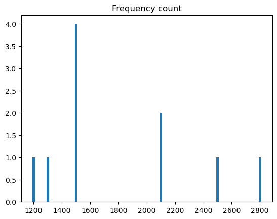
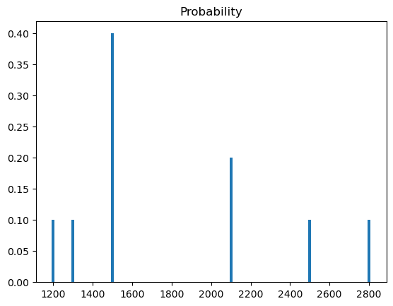
If we are asked what percentage of times a salary of 1500 occurred in the dataset then we can answer 40% (Why: 4 out of 10 salaries were 1500)

With the above figures, we can answer questions like

What are the chances of a person having salary less than 1500 euros?
What are the chances of a personal having a salary of 2800 euros?

These are just a few examples. Data distribution helps to answer such questions.

In a simple term, data distribution is a function which maps the value occuring in the dataset to its corresponding likelihood of appearing in the dataset.

For example, \[P(1500) = .4\]

Important

   Once we have distribution function we do not need the dataset to answer questions like those mentioned above.

We have several well defined data distribution functions which can be utilized to model the data. These distributions are divided into two categories based on values of data, i.e., Discrete and Continuous.

In this blog post, we will cover six discrete data distributions, i.e., Bernoulli, Binomial, Geometric, Negative Binomial, Hypergeometric, and Piosson.

Before diving into different discrete distributions, we need to first understand a bit about Random Variable. In data modeling problems, we are often interested in a particular phenomenon/event, e.g., salary in our previous example. We model such events using random variables denoted as \(X\).

Important

A random variable is not like a typical variable instead it is a mapping that maps the phenomenon/event of our interest into a real number.

Random variables can take any values from the sample space (i.e., all different salaries of employees, e.g., \(X=1500\))

In the following sections, you would often see the notation \(P(X=x)\) that represents the probability of random variable \(X\) to have a value \(x\).

Bernoulli distribution

This distribution is used to model a situation where there are two possible outcomes and you are interested in knowing the chance of happening those outcomes.

Let’s take an example of a scenario where this distribution can be used. Consider a person applying for a job which can lead to an offer or a rejection. The event of interest (e.g., getting a job offer) is termed as success and the other one as failure. These terms are simply used to make it easy for statistical modeling and do not have the usual connotations of success and failure. The possible outcomes can be represented numerically as 1 (success) and 0 (failure), respectively.

This distribution has a single parameter, i.e., p (probability of success). Given the total sum of probabilities of all events (success and failure in our case) must be 1. It makes the probability of failure (q) equal to (1-p). The formula is given below as well.

\[\begin{align*} P(x) = \left\{ \begin {aligned} & p & x = 1 \\ & 1-p & x = 0 \end{aligned} \right. \end{align*}\] Here, \(p\) is the probability of success.

Let’s take our previous example: The person has 25% chances of getting a job given his education level and experiences. In that case, the value of p is .4 that makes q = 1-p = .6. Figure Figure 2 shows the bar chart for p and q.

Code

plt.bar([0,1],[.6,.4],color='green',alpha=.5,width=.5)
plt.xticks([0,1],[0,1])
plt.ylim([0,1])
plt.title('Bernaulli distribution')
plt.ylabel('Probability')
plt.xlabel('Outcomes')
plt.show()

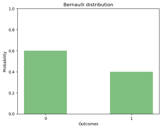
Let’s move to the two important properties of this distribution, i.e., expectation and variance. The expectation tells us which value we are going to observe on average in the Bernoulli distribution. The variance tells us how much deviation in general we notice in the distribution from the expected value.

\[ E[X] = p \] \[ Var[X] = pq \]

Let’s extend our example of job application.

Now, we are interested in knowing the chances of getting a particular number of job offers after applying for N job positions.

Here comes our next data distributions, Binomial distribution.

Binomial distribution

The binomial distribution is used to model a situation where N Bernoulli trials are performed. In other words, we have an event with two possible outcomes (0 and 1) and the event is repeated N times.

The binomial distribution is characterized by two parameters, \(N\) and \(\theta\) (or \(p\)). N is the number of trials, and \(\theta\) is the probability of ‘success’ or \(x=1\).

Consider our previous example of job applications. A person with a 30% chance of getting a job sent 10 job applications. We are interested in knowing what are the odds that that person would get 5 job offers.

Here, \(N = 10\) and \(p = .3\)

Now, we need to compute the probability of that person getting 5 job offers out of 10 job applications.

Let’s move to the formula for computing this probability. The formula in simple terms is given below. Here, \(X\) is number of job offers the person gets.

Important

\(P(X=x)\) = Number of ways event can occur * P(one occurrence)

In our example, the outcome resulting in getting the job corresponds to success while getting a rejection correspond to failure. Now, there could be a number of ways in which the results of 10 job applications could be. The following one is just one of them of our interest (5 successes).

         S S S S S F F F F F

We know that \(p = .3\) (previously mentioned that the person has 30% chance) that makes \(q = 1 - p = .7\). Now, in the above sequence of outcomes, there are 5 successes and 5 failures. The probability would be

\[ P = p*p*p*p*p*q*q*q*q*q \] \[ P = p^5 * q^5 \] \[ P = p^r * q^{n-r}\]

Here, r is the number of success

Now, we just need to find out how many ways are there in which there are 5 successes (e.g., another way could be S S S S F F F S F F). Here, we will use the following known as “n choose r”.

\[ \left( \begin {aligned} n \\ r \end{aligned} \right) = \frac{n!}{r!\,(n-r)!} \]

Here, \(!n\) is factorial of \(n\) defined as \[ !n = n * (n-1) * (n-2) * ... 2 * 1 \]

Now, we have knowledge on how may outcomes are there having r successes, and what is the probability of each of those outcomes. The following is the formula for Binomial distribution

\[ \left( \begin {aligned} n \\ r \end{aligned} \right) p^r * q^{n-r}\]

Let’s put the values in the formula for computing the probability of getting 5 job offers out of 10 with \(p=.3\).

\[ \left( \begin {aligned} 10 \\ 5 \end{aligned} \right) .3^5 * .7^5 \] \[ 252 * .0024 * .16 \] \[ .09 \]

There is 9% chances that the candidate will get 5 job offers out of 10 job application with \(p=.3\).

The expectation and variance of the Binomial distribution is given by

\[ E[X] = np \] \[ Var[X] = npq \]

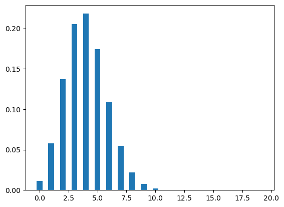
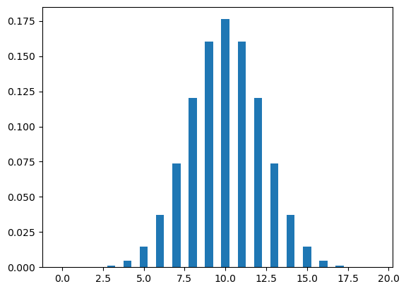
Let’s now plot the binomial distribution. The figure Figure 3 shows two different binomial distributions, one with p=.2 and other with p=.5. A binomial distribution with \(p=.5\) is symmetrical.

Code

def binomial_p(n,p,r):
    number_of_ways = math.factorial(n)/(math.factorial(r)*math.factorial(n-r))
    success_p = pow(p,r)
    failure_p = pow((1-p),(n-r))
    return number_of_ways * success_p * failure_p

def plot_binomial(n,p):
    x_data = []
    y_data = []
    
    for i in range(n):
        x_data.append(i)
        y_data.append(binomial_p(n,p,i))
        
    plt.bar(x_data,y_data,width=.5)
    #plt.title(f'n={n} p={p}')
    plt.show()

Code

plot_binomial(20,.2)
plot_binomial(20,.5)

Now, let’s say we are interested in knowing the number of rejection the candidate will face before getting the first job. What is the chance of the candidate to have a particular number of rejection before getting a job?.

Here comes our next distribution into the picture, the Geometric distribution.

Geometric distribution

The geometric distribution is used in situations where we like to model the number of failures (k) before the first success in a sequence of trials where each trial has two possible outcomes and the probability of those outcomes remains the same throughout the trials.

Important

Geometric distribution can also be used to model number of trials to get first success.

Let’s take our job example again.

Now, we would like to model how many rejections the candidate faces before getting a job offer. We will compute the probability for different cases, e.g., getting a job offer without any rejection, with 1 rejection, 2 rejections, and so on. In this case, our random variable X is number of rejections before first success.

In our example, the probability of getting a job is \(p = .3\), and getting a rejection is \(q=.7\).

Let’s now see the probabilities. There are cases in which the candidate gets the first job offer in the first application (S) or in the first attempt failure with success in the second attempt, and so on. The probabilities will be \[ P(S) = P(failures=0) = p \] \[ P(FS) = P(failures=1) = q * p \] \[ P(FFS) = P(failures=2) = q^2 * p \] \[ P(FFFS) = P(failures=3) = q^3 * p \]

We can generalize it in the following way

\[ P(failures=k) = q^{k} * p \]

The above equation gives us the probability of getting k failures before first success.

Tip

The probability sequence above is a geometric sequence where subsequent items have the same ratio. For example, \(a,a^2,a^3,a^4,...\). That is the reason why this distribution is called geometric distribution.

The expectation and variance of the Geometric distribution is given by (X is a random variable representing the number of failures before getting first success)

\[ E[X] = \frac{1-p}{p} \] \[ Var[X] = \frac{1-p}{p^2} \]

Tip

The Geometric distribution is also used to model number of trials in getting first success (let’s present it by a random variable Y). The total number of trials in getting first success is one more than the number of failures getting the first success. Therefore, the expecation value for this case would be

\[E[Y] = E[X] + 1 \] \[E[Y] = \frac{1}{p} \]

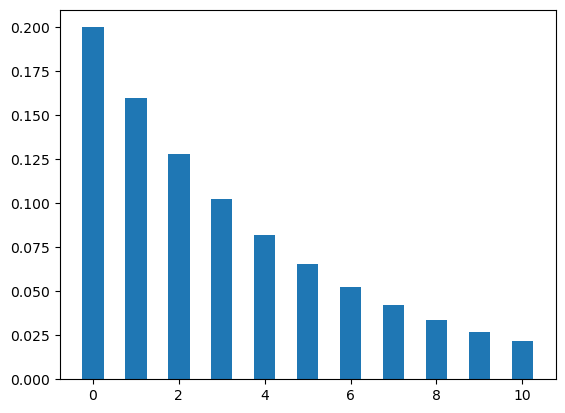
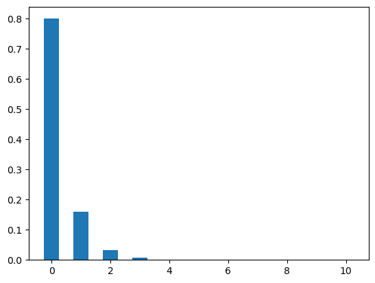
Let’s plot the geometric distribution. The figure Figure 4 shows two cases of geometric distributions. In the first case, the value of p is .2 which means the candidate has 20% chance of getting an offer for a job application. In the second case, the candidate has 80% chance for the same (that means p = .8).

The plots show the probability of getting different numbers of rejections before getting first offer.

Code

def geo_p(k,p):
    success_p = p
    failure_p = pow((1-p),(k))
    return success_p * failure_p

def plot_geo(n,p):
    x_data = []
    y_data = []
    
    for i in range(0,n+1):
        x_data.append(i)
        y_data.append(geo_p(i,p))
    plt.bar(x_data,y_data,width=.5)
    
    #plt.title(f'n={n} p={p}')
    plt.show()

Code

plot_geo(10,.2)
plot_geo(10,.8)

What about the probability of getting k rejections before getting rth job offer. We can answer this question with our next distribution.

Negative Binomial distribution

The negative binomial distribution used to model number of failures before getting r successes. Let’s take our previous example here. A person has a chance of 30% getting a job offer and his chance stays constant. Now, we are interested in knowing the probability of how many job rejections he would face before getting 3th job offer.

There can be multiple ways in which the candidate can get three job offers (some of them are listed below) S: job offer, R: rejection

No rejection  (k=0)   = S S (S)
One rejection (k=1)   = R S S (S) or S R S (S) or S S R (S)
Two rejection (k=2)   = R R S S (S) or R S S R S (S) or S S R R (S) ....

If we look at above sequences then we can see that the final occurrence is the 3rd success (job offer in our case). Before that there would be r-1 successes and k failures (k could be 0 1 2 3 ..). The formula for negative binomial then is

P(k) = probability of getting r-1 successes and k failure * probability of one success 
P(k) = probability of getting r-1 successes and k failure * p                      (1)

To compute the first part, we would use the formula from binomial distribution which gives us the probability of r success in n trials. In our case the total trials would be (r-1+k). That means the probability of getting r-1 successes in r-1+k trials would be

\[ \left( \begin {aligned} r-1+k \\ r-1 \end{aligned} \right) p^{r-1} * q^{k}\]

Now, we have probability of getting r-1 success and k failure. We will put it in our equation (1)

\[ P(k) = \left( \begin {aligned} r-1+k \\ r-1 \end{aligned} \right) p^{r-1} * q^{k} * p\]

\[ P(k) = \left( \begin {aligned} r-1+k \\ r-1 \end{aligned} \right) p^{r} * q^{k} \]

Tip

Why Negative?: In binomial distribution we model number of successes while with negative binomial we model number of failures.

The expectation and variance of the negative binomial (X representing number of failures before getting rth success )

\[ E[X] = \frac{r(1-p)}{p} \] \[ Var[X] = \frac{r(1-p)}{p^2} \]

Tip

The Negative binomial distribution is also used to model number of trials in getting rth success (let’s present it by a random variable Y). The total number of trials in getting r success is equal to the number of failures getting the rth success + r. Therefore, the expecation value for this case would be

\[E[Y] = E[X] + r \] \[E[Y] = \frac{r(1-p)}{p} + r \] \[E[Y] = \frac{r}{p}\]

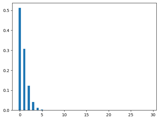
Let’s plot the negative binomial distribution. The figure Figure 5 shows two cases of binomial distributions. In the first case, the value of p is .2 which means the candidate has 20% chance of getting an offer for a job application. In the second case, the candidate has 80% chance for the same (that means p = .8).

Code

import math
def neg_p(p,r,k):
    success_p = pow(p,r)
    failure_p = pow((1-p),k)
    number_of_ways = math.factorial(r-1+k)/(math.factorial(r-1)*math.factorial(k))
    return number_of_ways * success_p * failure_p

def plot_neg(n_k,p,r):
    x_data = []
    y_data = []
    
    for i in range(0,n_k):
        x_data.append(i)
        y_data.append(neg_p(p,r,i))
    plt.bar(x_data,y_data,width=.5)
    #plt.title(f'n={n} p={p}')
    plt.show()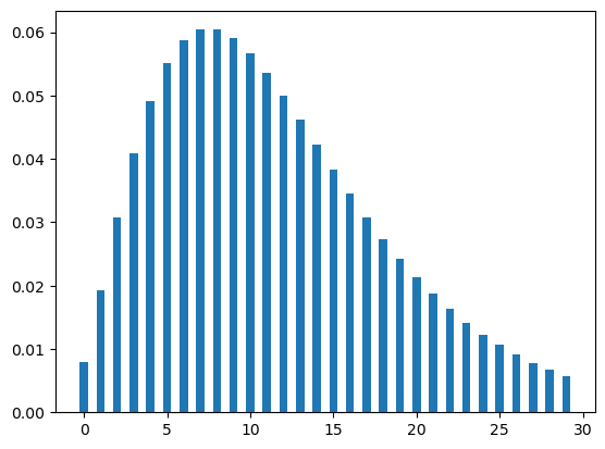

Code

plot_neg(30,.2,3)
plot_neg(30,.8,3)

Hypergeometric distribution

This distribution is different from all the aforementioned ones on the condition that p remains constant. In the previous distribution, our p (probability of success) remains constant across different trials. However, in hypergeometric this is not the case. To illustrate let’s take an example.

An organization wants to form a group to make a committee of 4 people (2 male, 2 female) out of 10 people (4 male, 6 female). In this example, with every selection the population changes. For example, the first section of a male employee would change the population from 10 (4 male, 6 female) to 9 (3 male, 6 female). This population change also affects the probability as well. The hypergeometric distribution is used to model such situations where sampling is done without replacement.

In this example, total number of population is N=10. There are K=4 male and N-K=6 female. In the sample, we need to select n=4 people, k=2 male and n-k= 2 female.

\[ \frac{\left( \begin {aligned} K \\ k \end{aligned} \right) * \left( \begin {aligned} N-K \\ n-k \end{aligned} \right)}{\left( \begin {aligned} N \\ n \end{aligned} \right)} \]

The hypergeometric distribution is characterised by (n,k, K, N) where

n : sample size or number of trials

k : number of success in sample or in n trials

K : number of success in population

N : population size

Code

def hyp_p(n,k,K,N):
    """
    N: Total number of events
    K: Number of success in population
    k: Number of success in sample
    n: Sample size/ number of trials
    """
    
    selection_K_k = math.factorial(K)/(math.factorial(k)*math.factorial(K-k))
    selection_N_minus_K = math.factorial(N-K)/(math.factorial(n-k) * math.factorial(N-K-n+k))
    selection_N_n = math.factorial(N)/(math.factorial(n) * math.factorial(N-n))
    return (selection_K_k * selection_N_minus_K)/selection_N_n

def plot_hyp(n,K,N):
    x_data = []
    y_data = []
    
    for i in range(1,n):
        x_data.append(i)
        y_data.append(hyp_p(n,i,K,N))
    plt.bar(x_data,y_data,width=.5)
    #plt.title(f'n={n} p={p}')
    plt.show()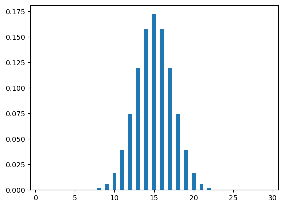

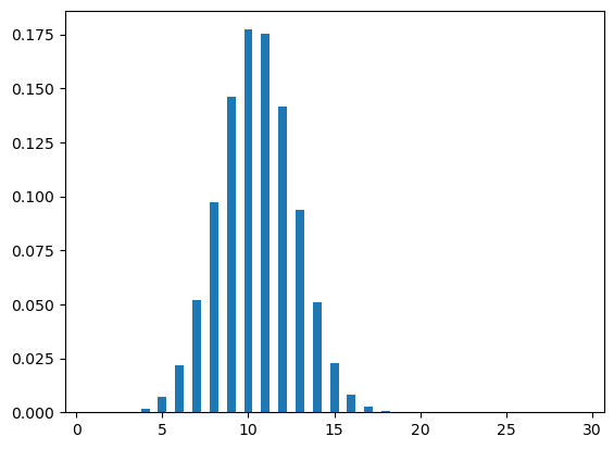
Code

plot_hyp(30,50,100)
plot_hyp(30,35,100)

Poisson distribution

Let’s now change our stance from employee to employer. An employer has an open job position and started receiving job applications. Every day the employer gets a particular number of applications and to process those applications the employer needs to make some arrangements.

To arrange for an upcoming week, the employer is interested in knowing the number of expected job applications in the next week. This is where Poisson distribution comes into the picture.

The Poisson distribution is used to model the number of occurrences in a particular period or a space unit. This distribution is characterized by \(\lambda\) which is an average number of events. The probability of k occurrences of events for given \(\lambda\) is the following

\[ P(k) = \frac{\lambda^k * e^{-\lambda}}{k!}\]

Using the above formula, we can compute the probability of getting k=10 job applications in the next week if the company is receiving an average of 7 job applications every week.

\[ P(X=10) = \frac{7^10 * e^{-7}}{10!}\]

\[ P(X=10)= .07 \]

Tip

The expected value and variance of the Poisson distribution both are \(\lambda\).

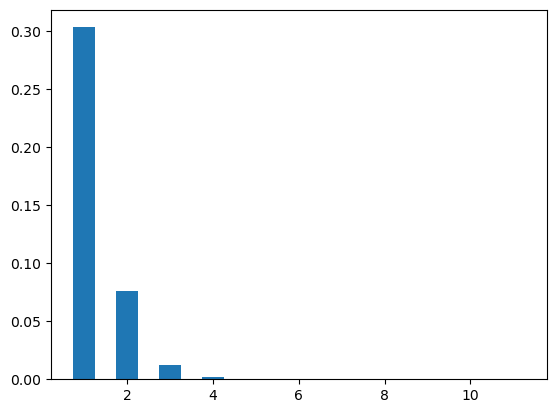
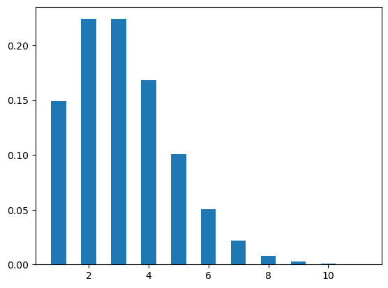
Figure Figure 7 shows two poisson distribution plots with different values of \(\lambda\), i.e., .5, 3.

Code

def poi_p(k,l):
    """
    k: number of occurences
    l: average number of occurences
    """
    return (pow(l,k)*math.exp(-l))/math.factorial(k)

def plot_poi(n,l):
    x_data = []
    y_data = []
    
    for i in range(1,n):
        x_data.append(i)
        y_data.append(poi_p(i,l))
    plt.bar(x_data,y_data,width=.5)
    #plt.title(f'n={n} p={p}')
    plt.show()

Code

plot_poi(12,.5)
plot_poi(12,3)

References

https://www3.nd.edu/~rwilliam/stats1/x13.pdf